Gallery of featured posts

Starting to think about AI Fairness
The topic of AI fairness metrics is as important to society as it is confusing. Confusing it is due to a number of reasons: terminological proliferation, abundance of formulae, and last not least the impression that everyone else seems to know what they're talking about. This text hopes to counteract some of that confusion by starting from a common-sense approach of contrasting two basic positions: On the one hand, the assumption that dataset features may be taken as reflecting the underlying concepts ML practitioners are interested in; on the other, that there inevitably is a gap between concept and measurement, a gap that may be bigger or smaller depending on what is being measured. In contrasting these fundamental views, we bring together concepts from ML, legal science, and political philosophy.

Beyond alchemy: A first look at geometric deep learning
Geometric deep learning is a "program" that aspires to situate deep learning architectures and techniques in a framework of mathematical priors. The priors, such as various types of invariance, first arise in some physical domain. A neural network that well matches the domain will preserve as many invariances as possible. In this post, we present a very conceptual, high-level overview, and highlight a few applications.

Introductory time-series forecasting with torch
This post is an introduction to time-series forecasting with torch. Central topics are data input, and practical usage of RNNs (GRUs/LSTMs). Upcoming posts will build on this, and introduce increasingly involved architectures.
Forecasting El Niño-Southern Oscillation (ENSO)
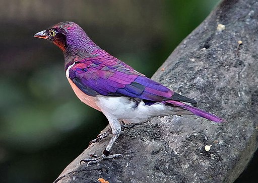
El Niño-Southern Oscillation (ENSO) is an atmospheric phenomenon, located in the tropical Pacific, that greatly affects ecosystems as well as human well-being on a large portion of the globe. We use the convLSTM introduced in a prior post to predict the Niño 3.4 Index from spatially-ordered sequences of sea surface temperatures.

Simple audio classification with torch
This article translates Daniel Falbel's post on "Simple Audio Classification" from TensorFlow/Keras to torch/torchaudio.
torch, tidymodels, and high-energy physics
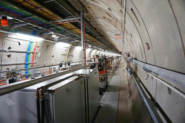
Today we introduce tabnet, a torch implementation of "TabNet: Attentive Interpretable Tabular Learning" that is fully integrated with the tidymodels framework. Per se, already, tabnet was designed to require very little data pre-processing; thanks to tidymodels, hyperparameter tuning (so often cumbersome in deep learning) becomes convenient and even, fun!

Convolutional LSTM for spatial forecasting
In forecasting spatially-determined phenomena (the weather, say, or the next frame in a movie), we want to model temporal evolution, ideally using recurrence relations. At the same time, we'd like to efficiently extract spatial features, something that is normally done with convolutional filters. Ideally then, we'd have at our disposal an architecture that is both recurrent and convolutional. In this post, we build a convolutional LSTM with torch.
Brain image segmentation with torch
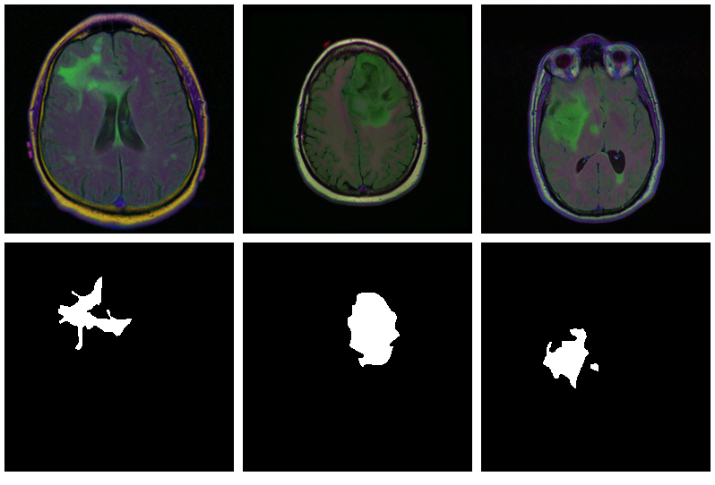
The need to segment images arises in various sciences and their applications, many of which are vital to human (and animal) life. In this introductory post, we train a U-Net to mark lesioned regions on MRI brain scans.

FNN-VAE for noisy time series forecasting
In the last part of this mini-series on forecasting with false nearest neighbors (FNN) loss, we replace the LSTM autoencoder from the previous post by a convolutional VAE, resulting in equivalent prediction performance but significantly lower training time. In addition, we find that FNN regularization is of great help when an underlying deterministic process is obscured by substantial noise.
Time series prediction with FNN-LSTM
In a recent post, we showed how an LSTM autoencoder, regularized by false nearest neighbors (FNN) loss, can be used to reconstruct the attractor of a nonlinear, chaotic dynamical system. Here, we explore how that same technique assists in prediction. Matched up with a comparable, capacity-wise, "vanilla LSTM", FNN-LSTM improves performance on a set of very different, real-world datasets, especially for the initial steps in a multi-step forecast.
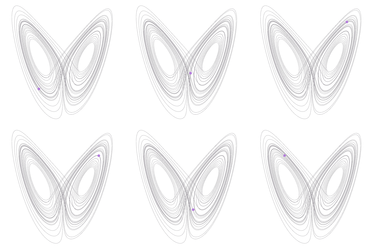
Deep attractors: Where deep learning meets chaos
In nonlinear dynamics, when the state space is thought to be multidimensional but all we have for data is just a univariate time series, one may attempt to reconstruct the true space via delay coordinate embeddings. However, it is not clear a priori how to choose dimensionality and time lag of the reconstruction space. In this post, we show how to use an autoencoder architecture to circumvent the problem: Given just a scalar series of observations, the autoencoder directly learns to represent attractors of chaotic systems in adequate dimensionality.
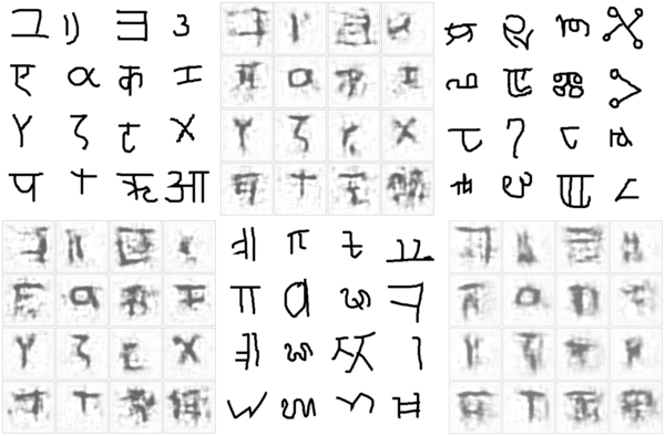
Hacking deep learning: model inversion attack by example
Compared to other applications, deep learning models might not seem too likely as victims of privacy attacks. However, methods exist to determine whether an entity was used in the training set (an adversarial attack called member inference), and techniques subsumed under "model inversion" allow to reconstruct raw data input given just model output (and sometimes, context information). This post shows an end-to-end example of model inversion, and explores mitigation strategies using TensorFlow Privacy.

Infinite surprise - the iridescent personality of Kullback-Leibler divergence
Kullback-Leibler divergence is not just used to train variational autoencoders or Bayesian networks (and not just a hard-to-pronounce thing). It is a fundamental concept in information theory, put to use in a vast range of applications. Most interestingly, it's not always about constraint, regularization or compression. Quite on the contrary, sometimes it is about novelty, discovery and surprise.
Getting started with Keras from R - the 2020 edition
Looking for materials to get started with deep learning from R? This post presents useful tutorials, guides, and background documentation on the new TensorFlow for R website. Advanced users will find pointers to applications of new release 2.0 (or upcoming 2.1!) features alluded to in the recent TensorFlow 2.0 post.

Differential Privacy with TensorFlow
Differential Privacy guarantees that results of a database query are basically independent of the presence in the data of a single individual. Applied to machine learning, we expect that no single training example influences the parameters of the trained model in a substantial way. This post introduces TensorFlow Privacy, a library built on top of TensorFlow, that can be used to train differentially private deep learning models from R.
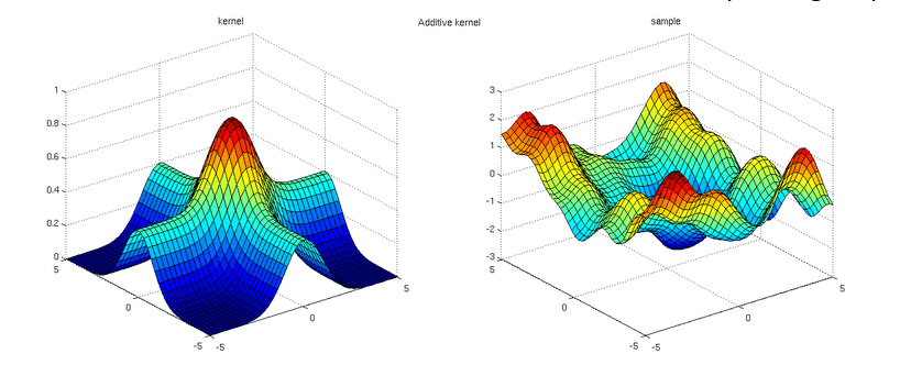
Gaussian Process Regression with tfprobability
Continuing our tour of applications of TensorFlow Probability (TFP), after Bayesian Neural Networks, Hamiltonian Monte Carlo and State Space Models, here we show an example of Gaussian Process Regression. In fact, what we see is a rather "normal" Keras network, defined and trained in pretty much the usual way, with TFP's Variational Gaussian Process layer pulling off all the magic.
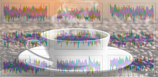
Hierarchical partial pooling, continued: Varying slopes models with TensorFlow Probability
This post builds on our recent introduction to multi-level modeling with tfprobability, the R wrapper to TensorFlow Probability. We show how to pool not just mean values ("intercepts"), but also relationships ("slopes"), thus enabling models to learn from data in an even broader way. Again, we use an example from Richard McElreath's "Statistical Rethinking"; the terminology as well as the way we present this topic are largely owed to this book.
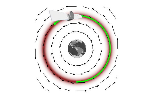
On leapfrogs, crashing satellites, and going nuts: A very first conceptual introduction to Hamiltonian Monte Carlo
TensorFlow Probability, and its R wrapper tfprobability, provide Markov Chain Monte Carlo (MCMC) methods that were used in a number of recent posts on this blog. These posts were directed to users already comfortable with the method, and terminology, per se, which readers mainly interested in deep learning won't necessarily be. Here we try to make up leeway, introducing Hamitonian Monte Carlo (HMC) as well as a few often-heard "buzzwords" accompanying it, always striving to keep in mind what it is all "for".
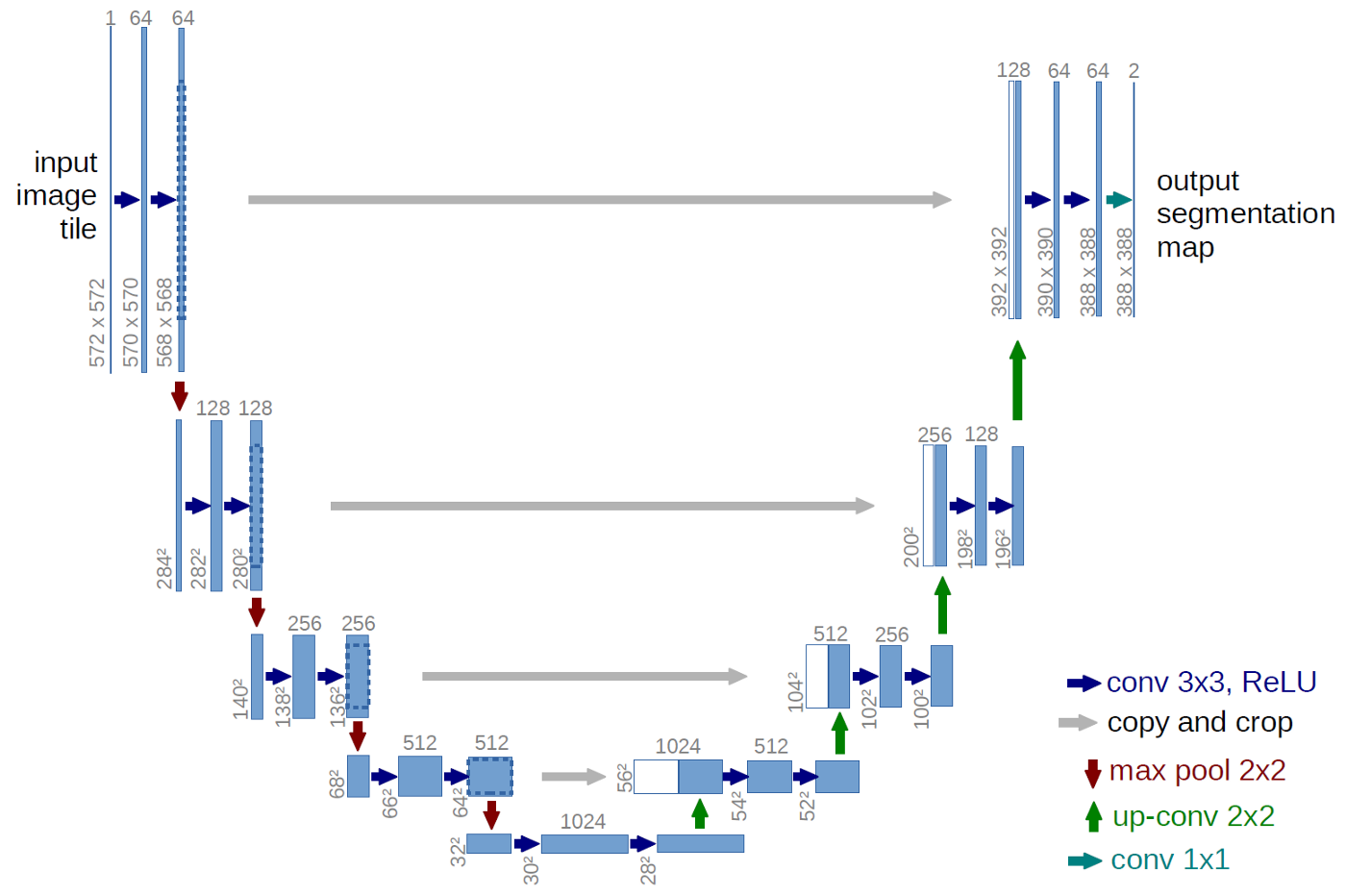
Image segmentation with U-Net
In image segmentation, every pixel of an image is assigned a class. Depending on the application, classes could be different cell types; or the task could be binary, as in "cancer cell yes or no?". Area of application notwithstanding, the established neural network architecture of choice is U-Net. In this post, we show how to preprocess data and train a U-Net model on the Kaggle Carvana image segmentation data.

Math, code, concepts: A third road to deep learning
Not everybody who wants to get into deep learning has a strong background in math or programming. This post elaborates on a concepts-driven, abstraction-based way to learn what it's all about.
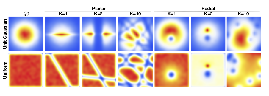
Getting into the flow: Bijectors in TensorFlow Probability
Normalizing flows are one of the lesser known, yet fascinating and successful architectures in unsupervised deep learning. In this post we provide a basic introduction to flows using tfprobability, an R wrapper to TensorFlow Probability. Upcoming posts will build on this, using more complex flows on more complex data.
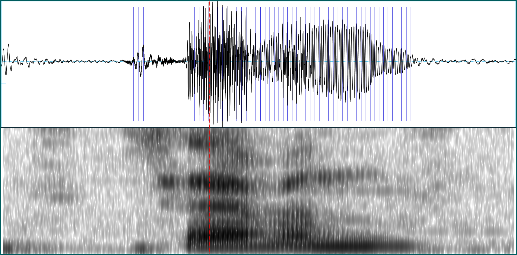
Audio classification with Keras: Looking closer at the non-deep learning parts
Sometimes, deep learning is seen - and welcomed - as a way to avoid laborious preprocessing of data. However, there are cases where preprocessing of sorts does not only help improve prediction, but constitutes a fascinating topic in itself. One such case is audio classification. In this post, we build on a previous post on this blog, this time focusing on explaining some of the non-deep learning background. We then link the concepts explained to updated for near-future releases TensorFlow code.
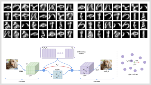
Discrete Representation Learning with VQ-VAE and TensorFlow Probability
Mostly when thinking of Variational Autoencoders (VAEs), we picture the prior as an isotropic Gaussian. But this is by no means a necessity. The Vector Quantised Variational Autoencoder (VQ-VAE) described in van den Oord et al's "Neural Discrete Representation Learning" features a discrete latent space that allows to learn impressively concise latent representations. In this post, we combine elements of Keras, TensorFlow, and TensorFlow Probability to see if we can generate convincing letters resembling those in Kuzushiji-MNIST.
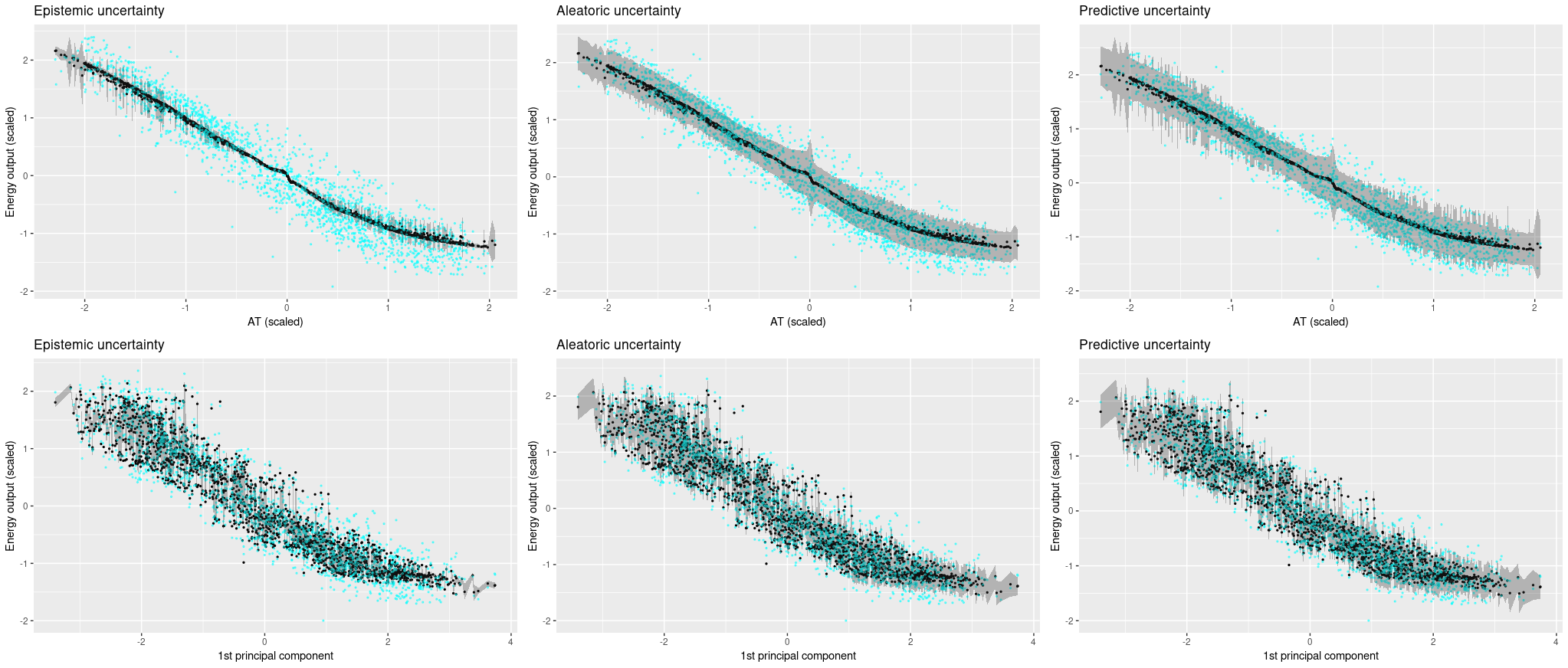
You sure? A Bayesian approach to obtaining uncertainty estimates from neural networks
In deep learning, there is no obvious way of obtaining uncertainty estimates. In 2016, Gal and Ghahramani proposed a method that is both theoretically grounded and practical: use dropout at test time. In this post, we introduce a refined version of this method (Gal et al. 2017) that has the network itself learn how uncertain it is.

Representation learning with MMD-VAE
Like GANs, variational autoencoders (VAEs) are often used to generate images. However, VAEs add an additional promise: namely, to model an underlying latent space. Here, we first look at a typical implementation that maximizes the evidence lower bound. Then, we compare it to one of the more recent competitors, MMD-VAE, from the Info-VAE (information maximizing VAE) family.

Collaborative filtering with embeddings
Embeddings are not just for use in natural language processing. Here we apply embeddings to a common task in collaborative filtering - predicting user ratings - and on our way, strive for a better understanding of what an embedding layer really does.

Attention-based Image Captioning with Keras
Image captioning is a challenging task at intersection of vision and language. Here, we demonstrate using Keras and eager execution to incorporate an attention mechanism that allows the network to concentrate on image features relevant to the current state of text generation.
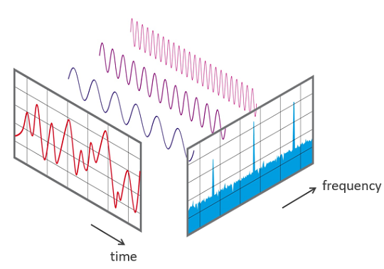
Simple Audio Classification with Keras
In this tutorial we will build a deep learning model to classify words. We will use the Speech Commands dataset which consists of 65,000 one-second audio files of people saying 30 different words.
Classifying physical activity from smartphone data
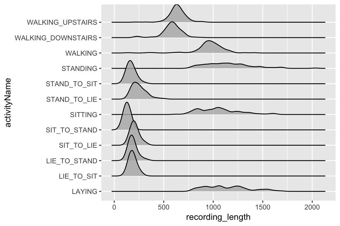
Using Keras to train a convolutional neural network to classify physical activity. The dataset was built from the recordings of 30 subjects performing basic activities and postural transitions while carrying a waist-mounted smartphone with embedded inertial sensors.

Attention-based Neural Machine Translation with Keras
As sequence to sequence prediction tasks get more involved, attention mechanisms have proven helpful. A prominent example is neural machine translation. Following a recent Google Colaboratory notebook, we show how to implement attention in R.

Predicting Fraud with Autoencoders and Keras
In this post we will train an autoencoder to detect credit card fraud. We will also demonstrate how to train Keras models in the cloud using CloudML. The basis of our model will be the Kaggle Credit Card Fraud Detection dataset.

Classifying Duplicate Questions from Quora with Keras
In this post we will use Keras to classify duplicated questions from Quora. Our implementation is inspired by the Siamese Recurrent Architecture, with modifications to the similarity measure and the embedding layers (the original paper uses pre-trained word vectors)
Deep Learning for Cancer Immunotherapy
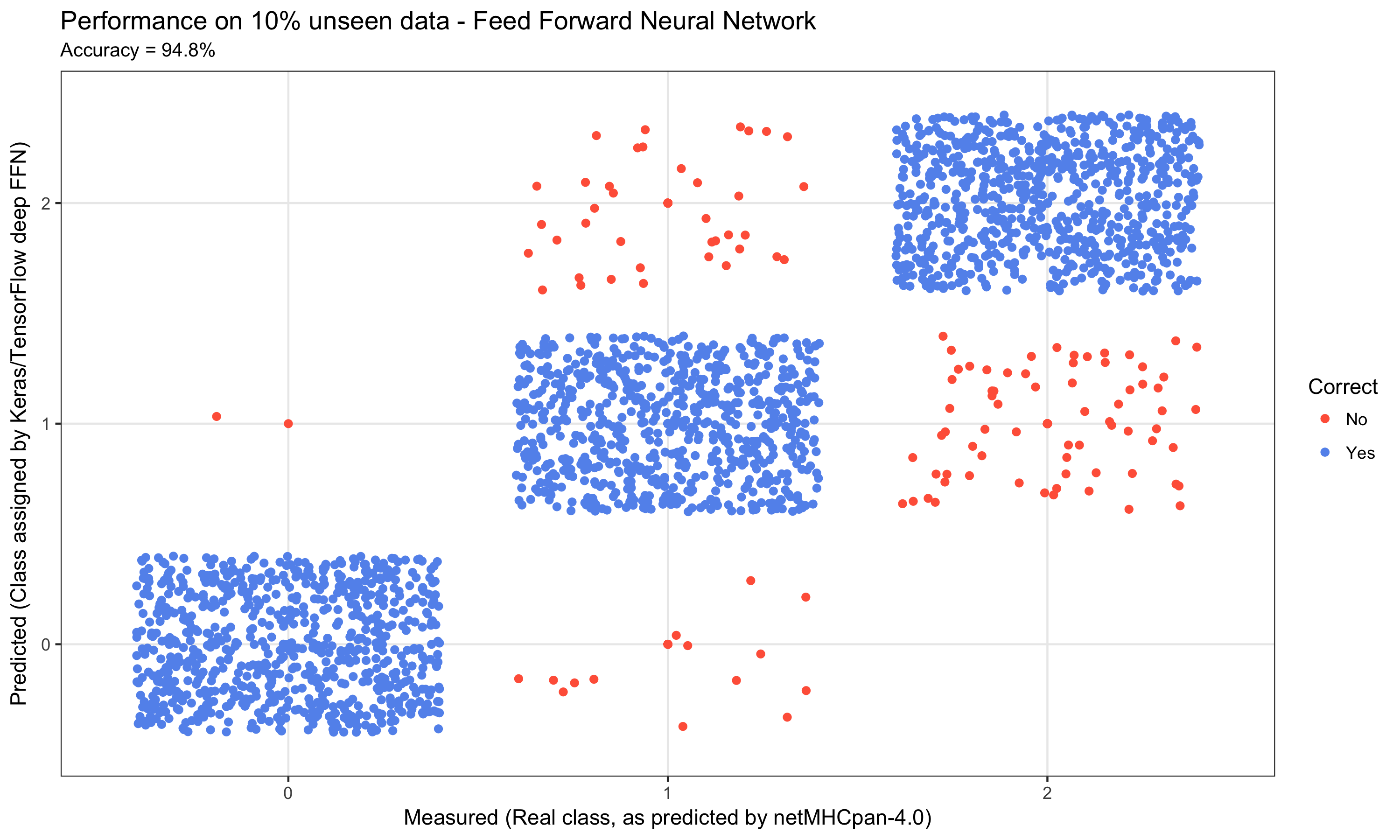
The aim of this post is to illustrate how deep learning is being applied in cancer immunotherapy (Immuno-oncology or Immunooncology) - a cancer treatment strategy, where the aim is to utilize the cancer patient's own immune system to fight the cancer.
Categories
- Articles (33)
- AI & Society (1)
- Audio Processing (3)
- Bayesian Modeling (2)
- Cloud (1)
- Concepts (7)
- Image Recognition & Image Processing (7)
- Meta (3)
- Natural Language Processing (3)
- Packages/Releases (1)
- Privacy & Security (2)
- Probabilistic ML/DL (5)
- R (12)
- Spatial Data (2)
- Tabular Data (3)
- TensorFlow/Keras (21)
- Time Series (7)
- Torch (6)
- Unsupervised Learning (7)